Difference between revisions of "GOES Flux vs STIX counts"
| (33 intermediate revisions by the same user not shown) | |||
| Line 1: | Line 1: | ||
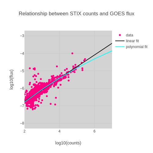
| − | [[File:Goes | + | [[File:Goes stix flux fit lms.png|800px|thumb|none| Scatter plot of STIX counts (4 - 10 keV) versus GOES and as well as a linear fit and a polynomial fit to the data. ]] |
| − | + | The GOES flux of a solar flare is estimated using<br> | |
| − | + | flux=10^(p0+p1*x), <br> | |
| + | with x=log10(stix_peak_counts*r^2)<br> | ||
| + | where p0, p1 are the parameters from the curve fit, peak_counts is the STIX QL LC peak | ||
| + | counts and r is the distance between the Sun and solar orbiter in units of au. <br> | ||
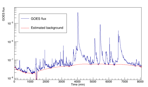
| − | + | [[File:Goes_background.png |600px|thumb|none| An example of estimated GOES flux background. ]] | |
| − | |||
| − | flux | ||
| − | |||
| − | |||
| − | |||
| − | |||
Latest revision as of 10:29, 21 January 2022
The GOES flux of a solar flare is estimated using
flux=10^(p0+p1*x),
with x=log10(stix_peak_counts*r^2)
where p0, p1 are the parameters from the curve fit, peak_counts is the STIX QL LC peak
counts and r is the distance between the Sun and solar orbiter in units of au.

